Calculus – Vector calculus – Green's theorem

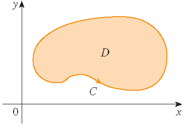
Definition: For a simple closed curve \(\mathcal{C}\) the positive orientation refers to a single counterclockwise traversal of \(\mathcal{C}\).

positive orientation	negative orientation

Definition: A region \(D\) in \(\mathbb{R}^2\) is called a regular region if it is both of type I and of type II.

Theorem: Let \(\mathcal{C}\) be a positively oriented, piecewise-smooth, simple closed curve in the plane and let \(D\) be the region bounded by \(\mathcal{C}\). If \(P\) and \(Q\) have continuous partial derivatives on an open region that contains \(D\), then

\[\oint\limits_{\mathcal{C}}P\,dx+Q\,dy=\iint\limits_D\left(\frac{\partial Q}{\partial x}-\frac{\partial P}{\partial y}\right)\,dA.\]

Note: Sometimes the notation \(\partial D\) is used for the positively oriented boundary curve of \(D\), that is: \(\mathcal{C}=\partial D\). Then

\[\iint\limits_D\left(\frac{\partial Q}{\partial x}-\frac{\partial P}{\partial y}\right)\,dA=\oint\limits_{\partial D}P\,dx+Q\,dy.\]

Proof (only for regular regions that are both of type I and type II): Note that the theorem will be proved if we can show that

\[\oint\limits_{\mathcal{C}}P\,dx=-\iint\limits_D\frac{\partial P}{\partial y}\,dA\quad\textrm{and}\quad \oint\limits_{\mathcal{C}}Q\,dy=\iint\limits_D\frac{\partial Q}{\partial x}\,dA.\]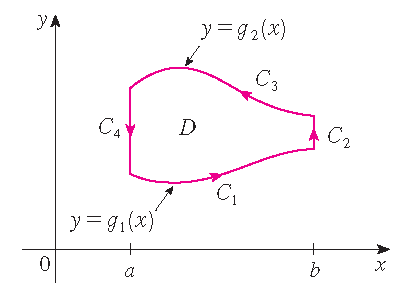

Since \(D\) is a type I region, we have: \(D=\{(x,y)\,|\,a\leq x\leq b,\;g_1(x)\leq y\leq g_2(x)\}\), where \(g_1\) and \(g_2\) are continuous functions. This enables us to evaluate the double integral \(\displaystyle\iint\limits_D\frac{\partial P}{\partial y}\,dA\):

\[\iint\limits_D\frac{\partial P}{\partial y}\,dA=\int_a^b\int_{g_1(x)}^{g_2(x)}\frac{\partial P}{\partial y}\,dy\,dx =\int_a^b\left(P(x,g_2(x))-P(x,g_1(x)\right)\,dx.\]

Now we evaluate the line integral \(\displaystyle\oint\limits_{\mathcal{C}}P\,dx\) by breaking up the curve \(\mathcal{C}\) as the union of four curves \(\mathcal{C}_1\), \(\mathcal{C}_2\), \(\mathcal{C}_3\) and \(\mathcal{C}_4\) as shown in the picture.

On \(\mathcal{C}_2\) and \(\mathcal{C}_4\) is \(x\) constant, so \(dx=0\), and therefore \(\displaystyle\int\limits_{\mathcal{C}_2}P(x,y)\,dx=0=\int\limits_{\mathcal{C}_4}P(x,y)\,dx\).

A parametrization of \(\mathcal{C}_1\) is \(\mathbf{r}(x)=x\,\mathbf{i}+g_1(x)\,\mathbf{j}\) with \(a\leq x\leq b\). Hence we have: \(\displaystyle\int\limits_{\mathcal{C}_1}P(x,y)\,dx=\int_a^bP(t,g_1(t))\,dt\). Furthermore, observe that a parametrization of \(-\mathcal{C}_3\) is \(\mathbf{r}(x)=x\,\mathbf{i}+g_2(x)\,\mathbf{j}\) with \(a\leq x\leq b\) and therefore \(\displaystyle\int\limits_{\mathcal{C}_3}P(x,y)\,dx=-\int\limits_{-\mathcal{C}_3}P(x,y)\,dx=-\int_a^bP(x,g_2(x))\,dx\). Hence we have:

\begin{align*} \oint\limits_{\mathcal{C}}P(x,y)\,dx&=\int\limits_{\mathcal{C}_1}P(x,y)\,dx+\int\limits_{\mathcal{C}_2}P(x,y)\,dx +\int\limits_{\mathcal{C}_3}P(x,y)\,dx+\int\limits_{\mathcal{C}_4}P(x,y)\,dx\\[2.5mm] &=\int_a^bP(x,g_1(x))\,dx+0-\int_a^bP(x,g_2(x))\,dx+0=\int_a^b\left(P(x,g_2(x))-P(x,g_1(x))\right)\,dx. \end{align*}

This implies that \(\displaystyle\oint\limits_{\mathcal{C}}P\,dx=-\iint\limits_D\frac{\partial P}{\partial y}\,dA\). In order to prove that \(\displaystyle\oint\limits_{\mathcal{C}}Q\,dy=\iint\limits_D\frac{\partial Q}{\partial x}\,dA\) we use that \(D\) is a type II region as well, which implies that \(D=\{(x,y)\,|\,c\leq y\leq d,\;h_1(y)\leq x\leq h_2(y)\}\), where \(h_1\) and \(h_2\) are continuous functions. Then we have:

\[\iint\limits_D\frac{\partial Q}{\partial x}\,dA=\int_c^d\int_{h_1(y)}^{h_2(y)}\frac{\partial Q}{\partial x}\,dx\,dy =\int_c^d\left(Q(h_2(y),y)-Q(h_1(y),y\right)\,dy.\]

Similarly, we evaluate the line integral \(\displaystyle\oint\limits_{\mathcal{C}}Q\,dy\) by breaking up the curve \(\mathcal{C}\) as the union of four curves \(\mathcal{C}_1\), \(\mathcal{C}_2\), \(\mathcal{C}_3\) and \(\mathcal{C}_4\), where \(y\) is constant on both \(\mathcal{C}_1\) and \(\mathcal{C}_3\) and therefore \(\displaystyle\int\limits_{\mathcal{C}_1}Q(x,y)\,dy=0=\int\limits_{\mathcal{C}_3}Q(x,y)\,dy\).

A parametrization of \(\mathcal{C}_2\) is \(\mathbf{r}(y)=h_2(y)\,\mathbf{i}+y\,\mathbf{j}\) with \(c\leq y\leq d\) and a parametrization of \(-\mathcal{C}_4\) is \(\mathbf{r}(y)=h_1(y)\,\mathbf{i}+y\,\mathbf{j}\) with \(c\leq y\leq d\) and therefore \begin{align*} \oint\limits_{\mathcal{C}}Q(x,y)\,dy&=\int\limits_{\mathcal{C}_1}Q(x,y)\,dy+\int\limits_{\mathcal{C}_2}Q(x,y)\,dy +\int\limits_{\mathcal{C}_3}Q(x,y)\,dy+\int\limits_{\mathcal{C}_4}Q(x,y)\,dy\\[2.5mm] &=0+\int_c^dQ(h_2(y),y)\,dy+0-\int_c^dQ(h_1(y),y)\,dy=\int_c^d\left(Q(h_2(y),y)-Q(h_1(y),y)\right)\,dy. \end{align*}

This implies that \(\displaystyle\oint\limits_{\mathcal{C}}Q\,dy=\iint\limits_D\frac{\partial Q}{\partial x}\,dA\).

Stewart §16.4, Example 1
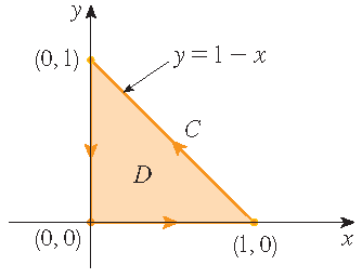
Evaluate \(\displaystyle\int\limits_{\mathcal{C}}x^4\,dx+xy\,dy\), where \(\mathcal{C}\) is the triangular curve consisting of the line segments from \((0,0)\) to \((1,0)\), from \((1,0)\) to \((0,1)\) and from \((0,1)\) to \((0,0)\) with positive orientation.

Solution: The line integral can be evaluated directly by using parametrizations of the three parts of the curve \(\mathcal{C}\). The line segment from \((0,0)\) to \((1,0)\) can be parametrized by \(\mathbf{r}(t)=\langle t,0 \rangle\) with \(0\leq t\leq 1\), the line segment from \((1,0)\) to \((0,1)\) by \(\mathbf{r}(t)=\langle 1-t,t \rangle\) with \(0\leq t\leq 1\) and the line segment from \((0,1)\) to \((0,0)\) by \(\mathbf{r}(t)=\langle 0,1-t \rangle\) with \(0\leq t\leq 1\). This leads to

\[\int\limits_{\mathcal{C}}x^4\,dx+xy\,dy=\int_0^1\left(t^4-(1-t)^4+t(1-t)+0\right)\,dt =\bigg[\frac{1}{5}t^5+\frac{1}{5}(1-t)^5+\frac{1}{2}t^2-\frac{1}{3}t^3\bigg]_{t=0}^1 =\frac{1}{5}+\frac{1}{2}-\frac{1}{3}-\frac{1}{5}=\frac{1}{6}.\]

Taking \(P(x,y)=x^4\) and \(Q(x,y)=xy\), the application of Green's theorem leads to

\[\int\limits_{\mathcal{C}}x^4\,dx+xy\,dy=\iint\limits_D\left(\frac{\partial Q}{\partial x}-\frac{\partial P}{\partial y}\right)\,dA =\int_0^1\int_0^{1-x}y\,dy\,dx=\int_0^1\bigg[\frac{1}{2}y^2\bigg]_{y=0}^{1-x}\,dx =\frac{1}{2}\int_0^1(1-x)^2\,dx=-\frac{1}{6}(1-x)^3\bigg|_{x=0}^1=\frac{1}{6}.\]

Stewart §16.4, Example 2
Evaluate \(\displaystyle\oint\limits_{\mathcal{C}}\left(3y-e^{\sin(x)}\right)\,dx+\left(7x+\sqrt{y^4+1}\right)\,dy\), where \(\mathcal{C}\) is the circle \(x^2+y^2=9\) with positive orientation.

Solution: The region \(D\) enclosed by the curve \(\mathcal{C}\) is the disk \(x^2+y^2\leq 9\). Using Green's theorem we obtain

\begin{align*} \oint\limits_{\mathcal{C}}\left(3y-e^{\sin(x)}\right)\,dx+\left(7x+\sqrt{y^4+1}\right)\,dy &=\iint\limits_D\left(\frac{\partial}{\partial x}\left(7x+\sqrt{y^4+1}\right)-\frac{\partial}{\partial y}\left(3y-e^{\sin(x)}\right)\right)\,dA\\[2.5mm] &=\iint\limits_D\left(7-3\right)\,dA=4\cdot\text{area}(D)=4\cdot9\pi=36\pi. \end{align*}

Computing areas

Since the area of a region \(D\) is equal to \(\displaystyle\iint\limits_D1\,dA\), we can apply Green's theorem as long as \(\displaystyle\frac{\partial Q}{\partial x}-\frac{\partial P}{\partial y}=1\) and find the area by evaluating a line integral over the positively oriented closed boundary curve \(\mathcal{C}\) that encloses \(D\). For instance, we have:

\[\text{area}(D)=\oint\limits_{\mathcal{C}}x\,dy=-\oint\limits_{\mathcal{C}}y\,dx=\tfrac{1}{2}\oint\limits_{\mathcal{C}}x\,dy-y\,dx.\]

Stewart §16.4, Example 3
Find the area of the region \(D\) enclosed by the ellipse \(\displaystyle\frac{x^2}{a^2}+\frac{y^2}{b^2}=1\) with \(a>0\) and \(b>0\).

Solution: A parametrization of the boundary curve \(\mathcal{C}\) is \(\mathbf{r}(t)=a\,\cos(t)\,\mathbf{i}+b\,\sin(t)\,\mathbf{j}\) with \(0\leq t\leq 2\pi\). Hence we have for instance

\[\text{area}(D)=\oint\limits_{\mathcal{C}}x\,dy=\int_0^{2\pi}a\,\cos(t)\,d\,b\,\sin(t)=ab\int_0^{2\pi}\cos^2(t)\,dt =\frac{1}{2}ab\int_0^{2\pi}\left(1+\cos(2t)\right)\,dt=\frac{1}{2}ab\bigg[t+\frac{1}{2}\sin(2t)\bigg]_{t=0}^{\pi}=ab\pi.\]

Similarly we have:

\[\text{area}(D)=-\oint\limits_{\mathcal{C}}y\,dx=-\int_0^{2\pi}b\,\sin(t)\,d\,a\,\cos(t)=ab\int_0^{2\pi}\sin^2(t)\,dt =\frac{1}{2}ab\int_0^{2\pi}\left(1-\cos(2t)\right)\,dt=\frac{1}{2}ab\bigg[t-\frac{1}{2}\sin(2t)\bigg]_{t=0}^{\pi}=ab\pi.\]

It is even nicer if we use the third fomula:

\[\text{area}(D)=\tfrac{1}{2}\oint\limits_{\mathcal{C}}x\,dy-y\,dx=\tfrac{1}{2}\int_0^{2\pi}\left(a\,\cos(t)\,d\,b\,\sin(t)-b\,\sin(t)\,d\,a\,\cos(t)\right) =\tfrac{1}{2}ab\int_0^{2\pi}\left(\cos^2(t)+\sin^2(t)\right)\,dt=ab\pi.\]

More general regions

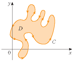
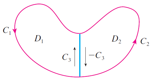
We have proved Green's theorem for regular regions \(D\) that are both of type I and of type II. It also holds for more general regions which can be written as a finite union of regular regions:

Note that the line integrals over the blue line segments in opposite directions cancel.

Stewart §16.4, Example 4
Evaluate \(\displaystyle\oint\limits_{\mathcal{C}}y^2\,dx+3xy\,dy\), where \(\mathcal{C}\) is the boundary of the semiannular region \(D\) in the upper half-plane between the circles \(x^2+y^2=1\) and \(x^2+y^2=4\).

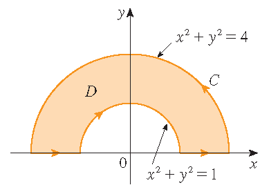
Solution: Note that \(D\) is of type I, but not of type II. However, the \(y\)-axis divides the region \(D\) into two parts which are both regular. This implies that Green's theorem may be applied. Using polar coordinates we obtain

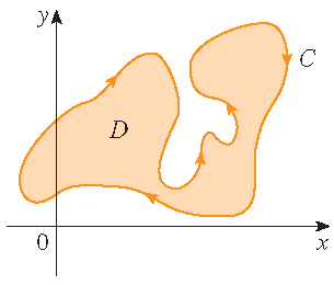
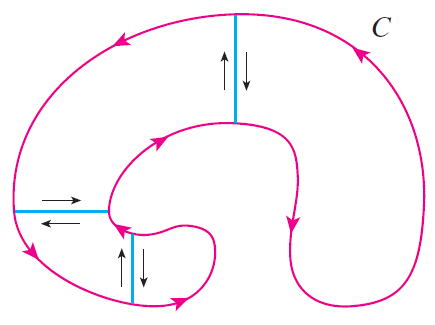
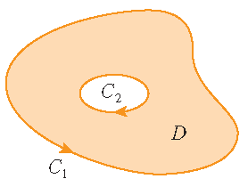
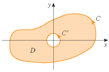
\begin{align*} \oint\limits_{\mathcal{C}}y^2\,dx+3xy\,dy&=\iint\limits_D\left(\frac{\partial}{\partial x}(3xy)-\frac{\partial}{\partial y}(y^2)\right)\,dA =\iint\limits_Dy\,dA=\int_0^{\pi}\int_1^2r\sin(\theta)\,r\,dr\,d\theta\\[2.5mm] &=\int_0^{\pi}\sin(\theta)\,d\theta\int_1^2r^2\,dr=\bigg[-\cos(\theta)\bigg]_{\theta=0}^{\pi}\cdot\bigg[\frac{1}{3}r^3\bigg]_{r=1}^2 =2\cdot\frac{7}{3}=\frac{14}{3}. \end{align*}

Green's theorem can be extended to apply to regions with holes, that is, regions that are not simply-connected. Observe that the boundary \(\mathcal{C}\) of the region \(D\) in the picture consists of two simple closed curves \(\mathcal{C}_1\) and \(\mathcal{C}_2\). We assume that these boundary curves are both oriented so that the region \(D\) is always on the left as the curve \(\mathcal{C}\) is traversed. Then the positive direction is counterclockwise for the outer curve \(\mathcal{C}_1\) and clockwise for the inner curve \(\mathcal{C}_2\).

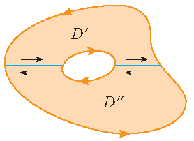Again we can divide the region \(D\) into two regions \(D'\) and \(D''\) as in the picture, where the line integrals over the blue segments in opposite directions cancel if we apply Green's theorem to both regions \(D'\) and \(D''\).

Stewart §16.4, Example 5
If \(\mathbf{F}(x,y)=-\displaystyle\frac{y}{x^2+y^2}\,\mathbf{i}+\frac{x}{x^2+y^2}\,\mathbf{j}\), show that \(\displaystyle\oint\limits_{\mathcal{C}}\mathbf{F}\cdot d\mathbf{r}=2\pi\) for every positively oriented simple closed curve \(\mathcal{C}\) that encloses the origin.

Solution: Since \(\mathcal{C}\) is an arbitrary closed curve that encloses the origin, it is impossible to evaluate the line integral directly. However, we can choose a counterclockwise oriented circle \(\mathcal{C}'\) with center the origin and radius \(\delta\), where \(\delta > 0\) is chosen to be small enough that \(\mathcal{C}'\) lies inside \(\mathcal{C}\). Let \(D\) be the region bounded by \(\mathcal{C}\) and \(\mathcal{C}'\). Then the positively oriented boundary of \(D\) is \(\mathcal{C}\cup\left(-\mathcal{C}'\right)\) and the general version of Green's theorem implies that

\[\oint\limits_{\mathcal{C}}P\,dx+Q\,dy+\oint\limits_{-\mathcal{C}'}P\,dx+Q\,dy =\iint\limits_D\left(\frac{\partial Q}{\partial x}-\frac{\partial P}{\partial y}\right)\,dA =\iint\limits_D\left(\frac{y^2-x^2}{(x^2+y^2)^2}-\frac{y^2-x^2}{(x^2+y^2)^2}\right)\,dA=0.\]

Note that \(D\) does not contain the origin. Hence we have

\[\oint\limits_{\mathcal{C}}\mathbf{F}\cdot d\mathbf{r}=\oint\limits_{\mathcal{C}}P\,dx+Q\,dy=-\oint\limits_{-\mathcal{C}'}P\,dx+Q\,dy =\oint\limits_{\mathcal{C}'}P\,dx+Q\,dy=\oint\limits_{\mathcal{C}'}\mathbf{F}\cdot d\mathbf{r}.\]

The latter line integral can be evaluated by using a parametrization of \(\mathcal{C}'\) which is \(\mathbf{r}(t)=\delta\,\cos(t)\,\mathbf{i}+\delta\,\sin(t)\,\mathbf{j}\) with \(0\leq t\leq 2\pi\). Hence we have

\[\oint\limits_{\mathcal{C}}\mathbf{F}\cdot d\mathbf{r}=\oint\limits_{\mathcal{C}'}\mathbf{F}\cdot d\mathbf{r} =\int_0^{2\pi}\langle -\frac{\delta\,\sin(t)}{\delta^2},\frac{\delta\,\cos(t)}{\delta^2} \rangle \cdot \langle -\delta\,\sin(t),\delta\,\cos(t) \rangle\,dt =\int_0^{2\pi}\left(\sin^2(t)+\cos^2(t)\right)\,dt=\int_0^{2\pi}dt=2\pi.\]

---

Last modified on October 13, 2021