Calculus – Functions of several variables – Functions of two variables

Definition: The maximal or natural domain \(D\) of a function \(f\) of two variables is the set of all points \((x,y)\) for which \(f(x,y)\) exists.

Remark: the actual domain of the function might a subset of this maximal or natural domain.

Definition: The range \(R\) of a function \(f\) of two variables is the set of all possible values of \(f(x,y)\), that is: \(R=\{f(x,y)\,|\,(x,y)\in D\}\).

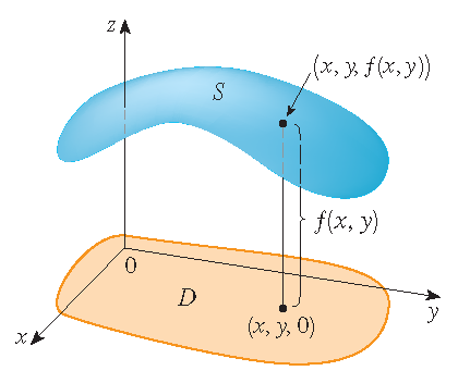
Definition: The graph of a function \(f\) of two variables with domain \(D\) is the set in \(\mathbb{R}^3\) of all points \((x,y,f(x,y))\) with \((x,y)\in D\).

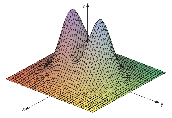
In general it is quite difficult to draw the graph of a function of two variables by hand:

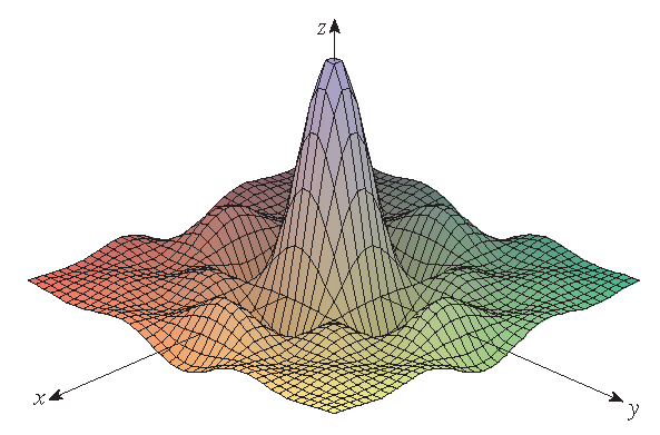the graph of \(f(x,y)=(x^2+3y^2)e^{-x^2-y^2}\)	the graph of \(g(x,y)=\displaystyle\frac{\sin(x)\sin(y)}{xy}\)

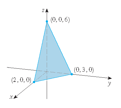
However, in some simple cases it is possible to draw the graph by hand:

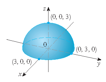the graph of \(f(x,y)=6-3x-2y\)	the graph of \(g(x,y)=\sqrt{9-x^2-y^2}\)

Definition: A level curve of a function \(f\) of two variables is a curve in \(\mathbb{R}^2\) with equation \(f(x,y)=k\), where \(k\) is a constant (in the range of \(f\)). A plot with several level curves is called a contour map.

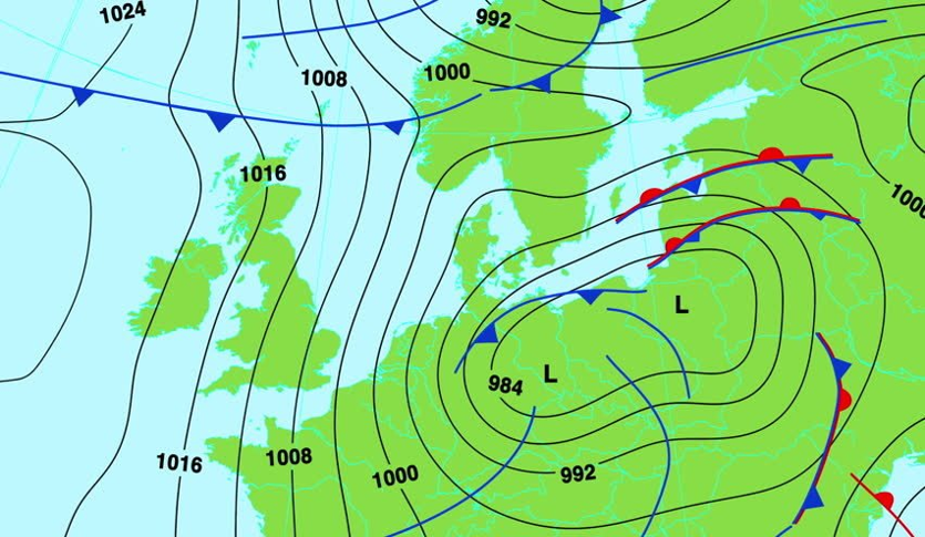
A contour map of atmospheric pressures over Central Europe

Examples of level curves:

1. constant elevations above sea level in topographic maps of mountaineous regions;


2. constant atmospheric pressure (isobars) in weather maps;


3. constant temperature (isothermals) in weather maps.

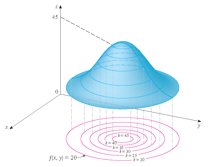
Level curves and the graph of a function:

Application:

Stewart §14.1: Exercise 39
The Body Mass Index (BMI) or Quetelet Index (QI) of a person is defined by

\[B(m,h)=\frac{m}{h^2},\]

where \(m\) is the person's mass (in kilograms) and \(h\) is the height (in meters).

The level curves \(B(m,h)=18\), \(B(m,h)=25\), \(B(m,h)=30\) and \(B(m,h)=40\) are drawn in the picture:

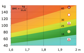
A rough guideline for the BMI is:

\[\begin{array}{|ccc|ccc|} \hline < 18 &:& \text{underweight} & 25 - 30 &:& \text{overweight}\\ 18 - 25 &:& \text{normal} & > 30 &:& \text{obese}\\ \hline \end{array}\]

So: the region corresponding to optimal BMI is green in the picture.

The BMI for a person who weighs \(62\) kg and is \(152\) cm tall is

\[B(62,1.52)=\frac{62}{(1.52)^2}\approx26.835.\]

This implies that the person is slightly overweight.

Stewart §14.1: Exercise 40
For a person who is \(200\) cm tall and weighs \(80\) kg the BMI equals

\[B(80,2)=\frac{80}{2^2}=20.\]

For a person of \(180\) cm tall with the same BMI we obtain:

\[B(m,1.8)=\frac{m}{(1.8)^2}=20\quad\Longrightarrow\quad m=20(1.8)^2=64.8.\]

For a person of \(170\) cm tall with the same BMI we obtain:

\[B(m,1.7)=\frac{m}{(1.7)^2}=20\quad\Longrightarrow\quad m=20(1.7)^2=57.8.\]

Conclusion: a person of \(180\) cm tall who weighs \(64.8\) kg and a person of \(170\) cm tall who weighs \(57.8\) kg have (exactly) the same BMI:

\[B(80,2)=B(64.8,1.8)=B(57.8,1.7)=20.\]

For a person who weighs \(70\) kg with the same BMI we obtain:

\[B(70,h)=\frac{70}{h^2}=20\quad\Longrightarrow\quad h^2=\frac{7}{2}\quad\Longrightarrow\quad h=\frac{1}{2}\sqrt{14}\approx1.87.\]

Conclusion: a person of \(187\) cm tall who weighs \(70\) kg has (approximately) the same BMI:

\[B(70,1.87)\approx20.\]

---

Last modified on September 15, 2021