Calculus – Functions of several variables – Partial derivatives

Definition: Let \(f\) be a function of two variables. Then

\[f_x(a,b)=\lim\limits_{h\to0}\frac{f(a+h,b)-f(a,b)}{h}\]

is called the partial derivative of \(f\) with respect to \(x\) at the point \((a,b)\) and

\[f_y(a,b)=\lim\limits_{h\to0}\frac{f(a,b+h)-f(a,b)}{h}\]

is called the partial derivative of \(f\) with respect to \(y\) at the point \((a,b)\).

More general: \(f_x(x,y)=\displaystyle\lim\limits_{h\to0}\frac{f(x+h,y)-f(x,y)}{h}\) and \(f_y(x,y)=\displaystyle\lim\limits_{h\to0}\frac{f(x,y+h)-f(x,y)}{h}\).

We use the notations

\[f_x(x,y)=f_x=\frac{\partial f}{\partial x}=\frac{\partial}{\partial x}f(x,y)\quad\text{and}\quad f_y(x,y)=f_y=\frac{\partial f}{\partial y}=\frac{\partial}{\partial y}f(x,y).\]

More than two variables

For a function \(f\) of three variables we have: \(f_x(x,y,z)=\displaystyle\lim\limits_{h\to0}\frac{f(x+h,y,z)-f(x,y,z)}{h}\), \(f_y(x,y,z)=\displaystyle\lim\limits_{h\to0}\frac{f(x,y+h,z)-f(x,y,z)}{h}\) and \(f_z(x,y,z)=\displaystyle\lim\limits_{h\to0}\frac{f(x,y,z+h)-f(x,y,z)}{h}\). Similarly in the case of more variables.

Higher-order partial derivatives

\begin{align*} f_{xx}&=(f_x)_x=\frac{\partial}{\partial x}\left(\frac{\partial f}{\partial x}\right)=\frac{\partial^2f}{\partial x^2}\\[2.5mm] f_{xy}&=(f_x)_y=\frac{\partial}{\partial y}\left(\frac{\partial f}{\partial x}\right)=\frac{\partial^2f}{\partial y\partial x}\\[2.5mm] f_{yx}&=(f_y)_x=\frac{\partial}{\partial x}\left(\frac{\partial f}{\partial y}\right)=\frac{\partial^2f}{\partial x\partial y}\\[2.5mm] f_{yy}&=(f_y)_y=\frac{\partial}{\partial y}\left(\frac{\partial f}{\partial y}\right)=\frac{\partial^2f}{\partial y^2} \end{align*}

Example: If \(f(x,y)=e^{2x+y}\ln(x^2+3y^2)\), then we have

\[f_x(x,y)=2e^{2x+y}\ln(x^2+3y^2)+e^{2x+y}\frac{2x}{x^2+3y^2}\quad\text{and}\quad f_y(x,y)=e^{2x+y}\ln(x^2+3y^2)+e^{2x+y}\frac{6y}{x^2+3y^2}.\]

Furthermore, we have

\[f_{xy}(x,y)=2e^{2x+y}\ln(x^2+3y^2)+2e^{2x+y}\frac{6y}{x^2+3y^2}+e^{2x+y}\frac{2x}{x^2+3y^2}-e^{2x+y}\frac{12xy}{(x^2+3y^2)^2}\]

and

\[f_{yx}(x,y)=2e^{2x+y}\ln(x^2+3y^2)+e^{2x+y}\frac{2x}{x^2+3y^2}+2e^{2x+y}\frac{6y}{x^2+3y^2}-e^{2x+y}\frac{12xy}{(x^2+3y^2)^2}.\]

Note that these are equal, which is not a coincidence.

Clairaut's theorem

Theorem: Suppose that \(f\) is defined on a disk \(D\) that contains the point \((a,b)\). If the functions \(f_{xy}\) and \(f_{yx}\) are both continuous on \(D\), then we have:

\[f_{xy}(a,b)=f_{yx}(a,b).\]

Proof: See Stewart, Appendix F.

Partial differential equations

Definition: A partial differential equation is an equation involving an unknown function of several variables and one or more of its partial derivatives.

Examples are

1. the heat conduction equation \(\alpha^2u_{xx}=u_t\) where \(\alpha^2\) denotes a positive constant (the thermal diffusivity);


2. the wave equation \(a^2u_{xx}=u_{tt}\), where \(a^2\) denotes a positive constant (the spring constant);


3. Laplace's (potential) equation \(u_{xx}+u_{yy}=0\).

Examples

1) The function \(u(x,y)=e^{-x}\cos(y)\) is a solution of Laplace's potential equation \(u_{xx}+u_{yy}=0\), since:

\[\left\{\begin{array}{l}u_x(x,y)=-e^{-x}\cos(y)\quad\Longrightarrow\quad u_{xx}(x,y)=e^{-x}\cos(y)\\[2.5mm] u_y(x,y)=-e^{-x}\sin(y)\quad\Longrightarrow\quad u_{yy}(x,y)=-e^{-x}\cos(y),\end{array}\right.\]

which implies that \(u_{xx}+u_{yy}=0\).

2) The function \(u(x,t)=\sin(x+at)\) is a solution of the wave equation \(a^2u_{xx}=u_{tt}\), since:

\[\left\{\begin{array}{l}u_x(x,t)=\cos(x+at)\quad\Longrightarrow\quad u_{xx}(x,t)=-\sin(x+at)\\[2.5mm] u_t(x,t)=a\cos(x+at)\quad\Longrightarrow\quad u_{tt}(x,t)=-a^2\sin(x+at),\end{array}\right.\]

which implies that \(a^2u_{xx}=u_{tt}\).

Application:

Stewart §14.3: Example 3
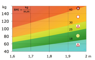
The Body Mass Index (BMI) or Quetelet Index (QI) of a person is defined by

\[B(m,h)=\frac{m}{h^2},\]

where \(m\) is the person's mass (in kilograms) and \(h\) is the height (in meters).

The partial derivatives of \(B\) with respect to \(m\) and \(h\) are: \(\displaystyle\frac{\partial B}{\partial m}=\frac{1}{h^2}\) and \(\displaystyle\frac{\partial B}{\partial h}=-\frac{2m}{h^3}\).

For instance:

\[B_m(64,1.68)=\frac{1}{(1.68)^2}\approx0.35\quad\text{and}\quad B_h(64,1.68)=-\frac{2\cdot64}{(1.68)^3}\approx-27.\]

So, for a person with a height of \(1.68\) m whose weight is \(64\) kg we have:

If the weight increases by a small amount, say \(1\) kg, and the height remains unchanged, then the BMI will increase by about \(0.35\).

If the height would increase by a small amount, say \(1\) cm, and the weight stays unchanged, then the BMI will decrease by about \(0.27\).

---

Last modified on September 15, 2021