Special Functions – Orthogonal polynomials

Definition: A sequence of polynomials \(\{p_n(x)\}_{n=0}^{\infty}\) with \(\text{degree}[p_n(x)]=n\) for each \(n\) is called orthogonal with respect to the weight function \(w(x)\) on the interval \((a,b)\) with \(a < b\) if

\[\int_a^bw(x)p_m(x)p_n(x)\,dx=h_n\,\delta_{mn}\quad\text{with}\quad\delta_{mn}:=\left\{\begin{array}{ll}0, & m\neq n\\[2.5mm]1, & m=n.\end{array}\right.\]

The weight function \(w(x)\) should be continuous and positive on \((a,b)\) such that the moments

\[\mu_n:=\int_a^bw(x)\,x^n\,dx,\quad n=0,1,2,\ldots\]

exist. Then the integral

\[\langle f,\,g\rangle:=\int_a^bw(x)f(x)g(x)\,dx\]

denotes an inner product of the polynomials \(f\) and \(g\). The interval \((a,b)\) is called the interval of orthogonality. This interval needs not to be finite.

If \(h_n=1\) for each \(n\in\{0,1,2,\ldots\}\) the sequence of polynomials is called orthonormal, and if

\[p_n(x)=k_nx^n+\;\text{lower order terms}\quad\text{with}\quad k_n=1\]

for each \(n\in\{0,1,2,\ldots\}\) the polynomials are called monic. The coefficient \(k_n\) is called the leading coefficient.

Starting with the sequence \(\{1,x,x^2,\ldots\}\) the Gram-Schmidt orthogonalization process can be used to construct the sequence of orthogonal polynomials.

Example: Let \(w(x)=1\) and \((a,b)=(0,1)\). Choose \(p_0(x)=1\). Then we have

\[p_1(x)=x-\frac{\langle x,\,p_0(x)\rangle}{\langle p_0(x),\,p_0(x)\rangle}\,p_0(x) =x-\frac{\langle x,\,1\rangle}{\langle 1,\,1\rangle}=x-\frac{1}{2},\]

since

\[\langle 1,\,1\rangle=\int_0^1\,dx=1\quad\text{and}\quad\langle x,\,1\rangle=\int_0^1x\,dx=\frac{1}{2}.\]

Further we have

\begin{align*} p_2(x)&=x^2-\frac{\langle x^2,\,p_0(x)\rangle}{\langle p_0(x),\,p_0(x)\rangle}\,p_0(x) -\frac{\langle x^2,\,p_1(x)\rangle}{\langle p_1(x),\,p_1(x)\rangle}\,p_1(x) =x^2-\frac{\langle x^2,\,1\rangle}{\langle 1,\,1\rangle} -\frac{\langle x^2,\,x-\textstyle\frac{1}{2}\rangle}{\langle x-\frac{1}{2},\,x-\frac{1}{2}\rangle}\left(x-\frac{1}{2}\right)\\[2.5mm] &=x^2-\frac{1}{3}-\left(x-\frac{1}{2}\right)=x^2-x+\frac{1}{6}, \end{align*}

since

\[\langle x^2,\,1\rangle=\int_0^1x^2\,dx=\frac{1}{3},\quad\langle x^2,\,x-{\textstyle\frac{1}{2}}\rangle =\int_0^1x^2\left(x-\frac{1}{2}\right)\,dx=\frac{1}{4}-\frac{1}{6}=\frac{1}{12}\]

and

\[\langle x-{\textstyle\frac{1}{2}},\,x-{\textstyle\frac{1}{2}}\rangle =\int_0^1\left(x-\frac{1}{2}\right)^2\,dx=\int_0^1\left(x^2-x+\frac{1}{4}\right)\,dx =\frac{1}{3}-\frac{1}{2}+\frac{1}{4}=\frac{1}{12}.\]

The polynomials \(p_0(x)=1\), \(p_1(x)=x-\frac{1}{2}\) and \(p_2(x)=x^2-x+\frac{1}{6}\) are the first three monic orthogonal polynomials on the interval \((0,1)\) with respect to the weight function \(w(x)=1\).

Repeating this process we obtain

\[p_3(x)=x^3-\frac{3}{2}x^2+\frac{3}{5}x-\frac{1}{20},\quad p_4(x)=x^4-2x^3+\frac{9}{7}x^2-\frac{2}{7}x+\frac{1}{70},\quad p_5(x)=x^5-\frac{5}{2}x^4+\frac{20}{9}x^3-\frac{5}{6}x^2+\frac{5}{42}x-\frac{1}{252},\]

and so on.

The orthonormal polynomials would be \(q_0(x)=p_0(x)/\sqrt{h_0}=1\), \(q_1(x)=p_1(x)/\sqrt{h_1}=2\sqrt{3}(x-1/2)\),

\[q_2(x)=\frac{p_2(x)}{\sqrt{h_2}}=6\sqrt{5}\left(x^2-x+\frac{1}{6}\right),\quad q_3(x)=\frac{p_3(x)}{\sqrt{h_3}}=20\sqrt{7}\left(x^3-\frac{3}{2}x^2+\frac{3}{5}x-\frac{1}{20}\right),\]

etcetera.

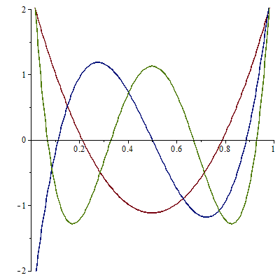
the polynomials \(q_2(x)\), \(q_3(x)\) and \(q_4(x)\).

---

Last modified on May 16, 2021