Linear Algebra – Systems of linear equations – Applications 2

Current flow in a simple electrical network can be described by a system of linear equations. A voltage source such as a battery forces a current of electrons to flow through the network. When the current passes through a resistor, some of the voltage is "used up"; by Ohm's law, this "voltage drop" across a resistor is given by \(V=RI\), where the voltage \(V\) is measured in volts, the resistance \(R\) in ohms (denoted by \(\Omega\)), and the current flow \(I\) in amperes.

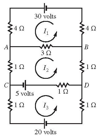
The network in the picture contains three closed loops. The currents flowing in the three loops are denoted by \(I_1\), \(I_2\) and \(I_3\). The designated directions are arbitrary; if a current turns out to be negative, then the actual direction is opposite to that chosen in the picture. If the current direction shown is away from the positive (longer) side of a battery around to the negative (shorter) side, the voltage is positive; otherwise, the voltage is negative.

Current flow in a loop is governed by the following rule:

Kirchhoff's voltage law
The algebraic sum of the \(RI\) voltage drops in one direction around a loop equals the algebraic sum of the voltage sources in the same direction around the loop.

Now we are able to determine the loop currents in the network in the picture:

For the first loop, the current \(I_1\) flows through three resistors, and the sum of the \(RI\) voltage drops is \(4I_1+4I_1+3I_1=11I_1\). Current from the second loop also flows in part of the first loop, through the branch between \(A\) and \(B\). The associated \(RI\) drop there is \(3I_2\) volts. However, the current direction for the branch \(AB\) in the first loop is ooposite to that chosen in the second loop, so the algebraic sum of all \(RI\) drops for the first loop is \(11I_1-3I_2\). Since the voltage in the first loop is \(30\) volts, Kirchhoff's voltage law implies that \(11I_1-3I_2=30\).

The equation for the second loop is: \(-3I_1+6I_2-I_3=5\). The term \(-3I_1\) comes from the current in the first loop through the branch \(AB\) with a negative voltage drop because the current flow there is opposite to the flow in the second loop. The term \(6I_2\) is the sum of all resistances in the second loop multiplied by the loop current. The term \(-I_3\) comes from the current in the third loop flowing through the \(1\)-ohm resistor in branch \(CD\), in the direction opposite to the flow in the second loop.

The equation for the third loop is: \(-I_2+3I_3=-25\). Note that the \(5\)-volt battery in branch \(CD\) is counted as part of both the second and third loop, but it is \(-5\) volts for the third loop because of the direction chosen for the current in the third loop. The \(20\)-volt battery is negative for the same reason.

Hence we have:

\[\left\{\begin{array}{rrrcr}11I_1&-3I_2&&=&30\\-3I_1&+6I_2&-I_3&=&5\\&-I_2&+3I_3&=&-25\end{array}\right.\quad\Longrightarrow\quad \left(\left.\begin{matrix}11&-3&0\\-3&6&-1\\0&-1&3\end{matrix}\,\right|\,\begin{matrix}30\\5\\-25\end{matrix}\right)\sim\;\cdots\;\sim \left(\left.\begin{matrix}1&0&0\\0&1&0\\0&0&1\end{matrix}\,\right|\,\begin{matrix}3\\1\\-8\end{matrix}\right).\]

The negative value of \(I_3\) indicates that the actual current in the third loop flows in the direction opposite to that chosen in the picture.

It is instructive to look at the system as a vector equation: \(I_1\begin{pmatrix}11\\-3\\0\end{pmatrix}+I_2\begin{pmatrix}-3\\6\\-1\end{pmatrix} +I_3\begin{pmatrix}0\\-1\\3\end{pmatrix}=\begin{pmatrix}30\\5\\-25\end{pmatrix}\). Note that the vectors on the left-hand side denote the resistances in the three loops; a resistance is written negatively when the corresponding current flows in the opposite direction of that in the corresponding loop. The vector on the right-hand side denotes the voltages in the three loops. If we define

\[R_1=\begin{pmatrix}11\\-3\\0\end{pmatrix},\quad R_2=\begin{pmatrix}-3\\6\\-1\end{pmatrix},\quad R_3=\begin{pmatrix}0\\-1\\3\end{pmatrix} \quad\text{and}\quad V=\begin{pmatrix}30\\5\\-25\end{pmatrix},\]

then we recognize Ohm's law in the matrix equation \(RI=V\), where \(R=\Bigg(R_1\;R_2\;R_3\Bigg)\) and \(I=\begin{pmatrix}I_1\\I_2\\I_3\end{pmatrix}\).

Difference equations

If \(A\) is a square matrix, then \(\mathbf{x}_{k+1}=A\mathbf{x}\) for \(k=0,1,2,\ldots\) is called a linear difference equation or recurrence relation. Given such an equation or relation, one can compute \(\mathbf{x}_1\), \(\mathbf{x}_2\), and so on, provided that \(\mathbf{x}_0\) is known.

Migration

A subject of interest to demographers is the movement of populations or groups of people from one region to another. The simple model here considers the changes in the population of a certain city and its surrounding suburbs over a period of years. Starting at a chosen initial year the initial population vector is \(\mathbf{x}_0=\begin{pmatrix}r_0\\s_0\end{pmatrix}\), where \(r_0\) denotes the city population and \(s_0\) the suburban population in that initial year. For the following years we denote the populations of the city and the suburbs by the vectors \(\mathbf{x}_1=\begin{pmatrix}r_1\\s_1\end{pmatrix}\), \(\mathbf{x}_2=\begin{pmatrix}r_2\\s_2\end{pmatrix}\), and so on. Our goal is to describe mathematically how these vectors might be related.

Suppose that demographic studies show that each year about \(6\%\) of the city's population moves to the suburbs, while \(4\%\) of the suburban population moves to the city. This implies that \(94\%\) of the city's population remains in the city and that \(96\%\) of the suburban populaltion remains in the suburbs. After one year, the original \(r_0\) persons in the city are now distributed between the city and the suburbs as \(\begin{pmatrix}0.94r_0\\0.06r_0\end{pmatrix}=r_0\begin{pmatrix}0.94\\0.06\end{pmatrix}\). The \(s_0\) persons in the suburbs in the initial year are distributed one year later as \(s_0\begin{pmatrix}0.04\\0.96\end{pmatrix}\). Hence we have:

\[\begin{pmatrix}r_1\\s_1\end{pmatrix}=r_0\begin{pmatrix}0.94\\0.06\end{pmatrix}+s_0\begin{pmatrix}0.04\\0.96\end{pmatrix} =\begin{pmatrix}0.94&0.04\\0.06&0.96\end{pmatrix}\begin{pmatrix}r_0\\s_0\end{pmatrix}.\]

Assuming that this pattern repeats, this leads to the difference equation \(\mathbf{x}_{k+1}=M\mathbf{x}_k\) for \(k=0,1,2,\ldots\), where \(M=\begin{pmatrix}0.94&0.04\\0.06&0.96\end{pmatrix}\) is called the migration matrix. Starting with \(\mathbf{x}_0=\begin{pmatrix}60000\\40000\end{pmatrix}\) we obtain: \(\mathbf{x}_1=M\mathbf{x}_0 =\begin{pmatrix}0.94&0.04\\0.06&0.96\end{pmatrix}\begin{pmatrix}60000\\40000\end{pmatrix}=\begin{pmatrix}58000\\42000\end{pmatrix}\),

\[\mathbf{x}_2=M\mathbf{x}_1=\begin{pmatrix}0.94&0.04\\0.06&0.96\end{pmatrix}\begin{pmatrix}58000\\42000\end{pmatrix} =\begin{pmatrix}56200\\43800\end{pmatrix},\quad\mathbf{x}_3=M\mathbf{x}_2=\begin{pmatrix}0.94&0.04\\0.06&0.96\end{pmatrix} \begin{pmatrix}56200\\43800\end{pmatrix}=\begin{pmatrix}54580\\45420\end{pmatrix},\quad\ldots.\]

Car rental company

Another example is a car rental company with three locations; one at the airport, one in the city center, and one in the suburbs. The policy is that a car rented at one location may be returned at any of the three locations. Research has shown that \(10\%\) of the cars rented at the airport were returned a the city center and \(5\%\) in the suburbs. Furthermore, \(10\%\) of the cars rented in the city center were returned at the airport and \(5\%\) in the suburbs. Finally, \(15\%\) of the cars rented in the suburbs were returned at the airport and \(5\%\) in the city center. We assume that the total amount of cars will stay the same.

Now we choose vectors with three entries in the order: airport, city center and suburbs. Then we have: \(\mathbf{x}_{k+1}=A\mathbf{x}_k\) for \(k=0,1,2,\ldots\) met

\[A=\begin{pmatrix}0.85&0.15&0.15\\0.10&0.80&0.05\\0.05&0.05&0.80\end{pmatrix}.\]

Each step might be a day or a week. Given a certain division of the vehicles among the three locations we are able to compute the changes. Suppose that the total amount of cars of the company equals \(100\) and that these are divided as follows among the three locations: \(40\) at the airport, \(30\) in the city center and \(30\) in the suburbs. Then the changes looks like this:

\[\mathbf{x}_0=\begin{pmatrix}40\\30\\30\end{pmatrix},\quad\mathbf{x}_1=A\mathbf{x}_0=\begin{pmatrix}0.85&0.15&0.15\\0.10&0.80&0.05\\0.05&0.05&0.80\end{pmatrix} \begin{pmatrix}40\\30\\30\end{pmatrix}=\begin{pmatrix}43.0\\29.5\\27.5\end{pmatrix},\quad\mathbf{x}_2=A\mathbf{x}_1 =\begin{pmatrix}0.85&0.15&0.15\\0.10&0.80&0.05\\0.05&0.05&0.80\end{pmatrix}\begin{pmatrix}43.0\\29.5\\27.5\end{pmatrix}=\begin{pmatrix}45.100\\29.275\\25.625\end{pmatrix},\quad\ldots.\]

Of course, the numbers of cars should be positive integers; alternatively one could consider the percentages of the total fleet instead. Later we will see that it is possible to describe the changes in detail and that we can predict what will be the division of the cars amnong the three locations in the future.

---

Last modified on March 22, 2021