Linear Algebra – Systems of linear equations – Applications 1

The closed Leontief input-output model in economics

A simple model of a small economy works as follows: suppose that the economy can be divided into three sectors \(A\), \(B\) and \(C\) and consider the input and the output of these sectors. We suppose that all output stays within the economy (closed model). Then for instance we have the following overview:

\[\begin{array}{|ccc|c|} \hline A&B&C&\\ \hline 0.0&0.6&0.3&A\\ 0.4&0.1&0.5&B\\ 0.6&0.3&0.2&C\\ \hline \end{array}\]

In each column it is displayed how the output of the corresponding sector is distributed over the three sectors. In each row it is displayed how much of the output of the three sectors is adopted by the corresponding sector.

The Russian economist Wassily Leontief (1906-1999) showed that there exists an equilibrium in the following sense: if we call the production of the three sectors \(P_A\), \(P_B\) and \(P_C\), then we demand that

\[P_A=0.6P_B+0.3P_C,\quad P_B=0.4P_A+0.1P_B+0.5P_C\quad\text{and}\quad P_C=0.6P_A+0.3P_B+0.2P_C.\]

This means: we are looking for a solution of the homogeneous system

\[\left\{\begin{array}{r}P_A-0.6P_B-0.3P_C=0\\-0.4P_A+0.9P_B-0.5P_C=0\\-0.6P_A-0.3P_B+0.8P_C=0\end{array}\right.\quad\Longrightarrow\quad \begin{pmatrix}1&-0.6&-0.3\\-0.4&0.9&-0.5\\-0.6&-0.3&0.8\end{pmatrix}\sim\begin{pmatrix}1&-0.6&-0.3\\0&0.66&-0.62\\0&-0.66&0.62\end{pmatrix} \sim\begin{pmatrix}1&-0.60&-0.30\\0&0.66&-0.62\\0&0&0\end{pmatrix}.\]

The general solution can be written as \(\begin{pmatrix}P_A\\P_B\\P_C\end{pmatrix}=k\begin{pmatrix}0.285\\0.310\\0.330\end{pmatrix}\) with \(k\) an arbitrary (positive) constant. We can choose this constant such that the sum of the entries of this vector equals the total production of the three sectors.

Another example is:

\[\begin{array}{|ccc|c|} \hline A&B&C&\\ \hline \frac{1}{2}&\frac{1}{3}&\frac{1}{4}&A\\ \frac{1}{4}&\frac{1}{3}&\frac{1}{4}&B\\ \frac{1}{4}&\frac{1}{3}&\frac{1}{2}&C\\ \hline \end{array}\]

In that case we have: \(P_A=\frac{1}{2}P_A+\frac{1}{3}P_B+\frac{1}{4}P_C\), \(P_B=\frac{1}{4}P_A+\frac{1}{3}P_B+\frac{1}{4}P_C\) and \(P_C=\frac{1}{4}P_A+\frac{1}{3}P_B+\frac{1}{2}P_C\) oftewetl:

\[\left\{\begin{array}{r}\frac{1}{2}P_A-\frac{1}{3}P_B-\frac{1}{4}P_C=0\\-\frac{1}{4}P_A+\frac{2}{3}P_B-\frac{1}{4}P_C=0\\ -\frac{1}{4}P_A-\frac{1}{3}P_B+\frac{1}{2}PC=0\end{array}\right.\quad\Longrightarrow\quad \begin{pmatrix}\frac{1}{2}&-\frac{1}{3}&-\frac{1}{4}\\-\frac{1}{4}&\frac{2}{3}&-\frac{1}{4}\\-\frac{1}{4}&-\frac{1}{3}&\frac{1}{2}\end{pmatrix} \sim\begin{pmatrix}\frac{1}{2}&-\frac{1}{3}&-\frac{1}{4}\\0&\frac{1}{2}&-\frac{3}{8}\\0&-\frac{1}{2}&\frac{3}{8}\end{pmatrix} \sim\begin{pmatrix}\frac{1}{2}&0&-\frac{1}{2}\\0&\frac{1}{2}&-\frac{3}{8}\\0&0&0\end{pmatrix}.\]

The general solution is \(\begin{pmatrix}P_A\\P_B\\P_C\end{pmatrix}=k\begin{pmatrix}4\\3\\4\end{pmatrix}\) with \(k\) an arbitrary (positive) constant. For instance, for \(k=\frac{1}{11}\) the total production is set to \(1\).

Balance in chemical equations

A chemical equations describes the numbers of molecules that are involved in a chemical reaction. For instance: when propane gas burns, the propane reacts with oxygen to form carbon dioxide and water:

\[x_1\,C_3H_8+x_2\,O_2\;\;\longrightarrow\;\;x_3\,CO_2+x_4\,H_2O.\]

In order to "balance" this equation, a chemist should find positive integers \(x_1\),\(x_2\), \(x_3\) en \(x_4\) such that the total numbers of carbon (C), hydrogen (H) and oxygen (O) atoms to the left and to the right should be equal. This can be done by writing this in terms of a vector equation, where the entries of the vectors indicate the numbers of carbon (C), hydrogen (H) and oxygen (O) atoms, respectively: \(\begin{pmatrix}C\\H\\O\end{pmatrix}\). Then we have:

\[x_1\begin{pmatrix}3\\8\\0\end{pmatrix}+x_2\begin{pmatrix}0\\0\\2\end{pmatrix}=x_3\begin{pmatrix}1\\0\\2\end{pmatrix} +x_4\begin{pmatrix}0\\2\\1\end{pmatrix}.\]

This leads to a homogeneous vector equation:

\[x_1\begin{pmatrix}3\\8\\0\end{pmatrix}+x_2\begin{pmatrix}0\\0\\2\end{pmatrix}-x_3\begin{pmatrix}1\\0\\2\end{pmatrix} -x_4\begin{pmatrix}0\\2\\1\end{pmatrix}=\mathbf{0}:\quad\begin{pmatrix}3&0&-1&0\\8&0&0&-2\\0&2&-2&-1\end{pmatrix} \sim\begin{pmatrix}4&0&0&-1\\0&4&0&-5\\0&0&4&-3\end{pmatrix}\quad\Longrightarrow\quad\left\{\begin{array}{l}x_1=\frac{1}{4}x_4\\ x_2=\frac{5}{4}x_4\\x_3=\frac{3}{4}x_4\\x_4\;\text{is free.}\end{array}\right.\]

Since we should have (positive) integers as solutions, we now choose \(x_4=4\) (for the smallest integers):

\[C_3H_8+5\,O_2\;\;\longrightarrow\;\;3\,CO_2+4\,H_20.\]

Another example is:

\[x_1\,NH_3+x_2\,O_2\;\;\longrightarrow\;\;x_3\,NO+x_4\,H_2O.\]

Then we have using vectors \(\begin{pmatrix}N\\H\\O\end{pmatrix}\):

\[x_1\begin{pmatrix}1\\3\\0\end{pmatrix}+x_2\begin{pmatrix}0\\0\\2\end{pmatrix}=x_3\begin{pmatrix}1\\0\\1\end{pmatrix}+x_4\begin{pmatrix}0\\2\\1\end{pmatrix}:\; \begin{pmatrix}1&0&-1&0\\3&0&0&-2\\0&2&-1&-1\end{pmatrix}\sim\begin{pmatrix}1&0&-1&0\\0&0&3&-2\\0&2&-1&-1\end{pmatrix} \sim\begin{pmatrix}1&0&0&-\frac{2}{3}\\0&2&0&-\frac{5}{3}\\0&0&1&-\frac{2}{3}\end{pmatrix}\;\Longrightarrow\; \left\{\begin{array}{l}x_1=\frac{2}{3}x_4\\x_2=\frac{5}{6}x_4\\x_3=\frac{2}{3}x_4\\x_4\;\text{is free.}\end{array}\right.\]

Now we obtain the smallest solution with (positive) integers if we take \(x_4=6\). So:

\[4\,NH_3+5O_2\;\;\longrightarrow\;\;4\,NO+6\,H_2O.\]

Network flows

Consider for instance the traffic flows in a road network, where at some locations the number of passing vehicles is counted. Taking into account the one way traffic, the numbers per hour are indicated in the picture.

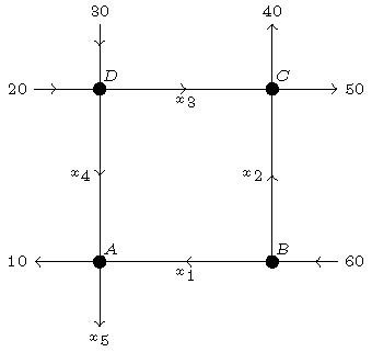
Using these data we are able to track down the complete pattern of the traffic flows. At each crossing or junction we set up an equilibrium equation; the number of incoming vehicles should be equal to the number of outgoing vehicles. Then we have:

\[\left\{\begin{array}{l}A:\;x_1+x_4=x_5+10\\[2.5mm]B:\;60=x_1+x_2\\[2.5mm]C:\;x_2+x_3=40+50\\[2.5mm]D:\;20+30=x_3+x_4\end{array}\right.\quad\Longrightarrow\quad \left\{\begin{array}{rrrrrcl}x_1&&&+x_4&-x_5&=&10\\[2.5mm]x_1&+x_2&&&&=&60\\[2.5mm]&x_2&+x_3&&&=&90\\[2.5mm]&&x_3&+x_4&&=&50.\end{array}\right.\]

This is a nonhomogeneous system of linear equations, so:

\[\left(\left.\begin{matrix}1&0&0&1&-1\\1&1&0&0&0\\0&1&1&0&0\\0&0&1&1&0\end{matrix}\,\right|\,\begin{matrix}10\\60\\90\\50\end{matrix}\right) \sim\;\;\cdots\;\;\sim\left(\left.\begin{matrix}1&0&0&1&0\\0&1&0&-1&0\\0&0&1&1&0\\0&0&0&0&1\end{matrix}\,\right|\,\begin{matrix}20\\40\\50\\10\end{matrix}\right) \quad\Longrightarrow\quad\left\{\begin{array}{l}x_1=20-x_4\\x_2=40+x_4\\x_3=50-x_4\\x_4\;\text{is free}\\x_5=10.\end{array}\right.\]

Since we have to deal with one way traffic, the variables may not be negative (then the traffic would be in the opposite direction). So we conclude that \(0\leq x_4\leq 20\). Note that this implies that \(0\leq x_1\leq 20\) too, \(40\leq x_2\leq 60\) and \(30\leq x_3\leq 50\).

Yet another example, again with one way traffic:

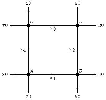
Now we obtain:

\[\left\{\begin{array}{l}A:\;30+x_4=20+x_1\\[2.5mm]B:\;60+x_1=40+x_2\\[2.5mm]C:\;80+x_2=50+x_3\\[2.5mm]D:\;10+x_3=70+x_4\end{array}\right.\quad\Longrightarrow\quad \left\{\begin{array}{rrrrcr}x_1&&&-x_4&=&10\\[2.5mm]-x_1&+x_2&&&=&20\\[2.5mm]&-x_2&+x_3&&=&30\\[2.5mm]&&-x_3&+x_4&=&-60\end{array}\right.\]

en dus

\[\left(\left.\begin{matrix}1&0&0&-1\\-1&1&0&0\\0&-1&1&0\\0&0&-1&1\end{matrix}\,\right|\,\begin{matrix}10\\20\\30\\-60\end{matrix}\right) \sim\;\;\cdots\;\;\sim\left(\left.\begin{matrix}1&0&0&-1\\0&1&0&-1\\0&0&1&-1\\0&0&0&0\end{matrix}\,\right|\,\begin{matrix}10\\30\\60\\0\end{matrix}\right) \quad\Longrightarrow\quad\left\{\begin{array}{l}x_1=10+x_4\\x_2=30+x_4\\x_3=60+x_4\\x_4\;\text{is free.}\end{array}\right.\]

---

Last modified on March 22, 2021