Calculus – Integration – Applications

The normal distribution

In probability and statistics the normal distribution plays an important role. This is based on the graph of the function \(e^{-x^2}\):

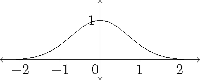
This graph is sometimes called a Gaussian curve or a bell curve. By symmetry we have \(\displaystyle\int_{-\infty}^{\infty}e^{-x^2}\,dx=2\int_0^{\infty}e^{-x^2}\,dx\).

In Stewart §7.8, Example 9 it is shown that this integral is convergent:

\[\int_0^{\infty}e^{-x^2}\,dx=\int_0^1e^{-x^2}\,dx+\int_1^{\infty}e^{-x^2}\,dx.\]

The first integral on the right-hand side is just an ordinary finite integral. In the second integral we use the fact that for \(x\geq1\) we have \(x^2\geq x\), so \(−x^2\leq-x\) and therefore \(e^{-x^2}\leq e^{-x}\). Now we have:

\[\int_1^{\infty}e^{-x}\,dx=\lim\limits_{t\to\infty}\int_1^te^{-x}\,dx=\lim\limits_{t\to\infty}\left(e^{-1}-e^{-t}\right)=e^{-1}.\]

This shows that the second integral converges.

Later we will prove that \(\displaystyle\int_0^{\infty}e^{-x^2}\,dx=\tfrac{1}{2}\sqrt{\pi}\), which implies that \(\displaystyle\int_{-\infty}^{\infty}e^{-x^2}\,dx=\sqrt{\pi}\). This is often called the Gaussian integral.

Of course, in probability and statistics it is essential that \(\displaystyle\frac{1}{\sqrt{\pi}}\int_{-\infty}^{\infty}e^{-x^2}\,dx=1\).

The Cauchy distribution

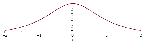
The Cauchy distribution is another probability distribution which is based on the graph of the function \(\displaystyle\frac{1}{1+x^2}\):

In Stewart §7.8, Example 3 this integral is evaluated:

\[\int_{-\infty}^{\infty}\frac{1}{1+x^2}\,dx=\int_{-\infty}^0\frac{1}{1+x^2}\,dx+\int_0^{\infty}\frac{1}{1+x^2}\,dx.\]

Now we have:

\[\int_0^{\infty}\frac{1}{1+x^2}\,dx=\arctan(x)\bigg|_0^{\infty}=\frac{1}{2}\pi-0=\frac{1}{2}\pi\quad\text{en}\quad \int_{-\infty}^0\frac{1}{1+x^2}\,dx=\arctan(x)\bigg|_{-\infty}^0=0-\left(-\frac{1}{2}\pi\right)=\frac{1}{2}\pi.\]

This implies that

\[\int_{-\infty}^{\infty}\frac{1}{1+x^2}\,dx=\frac{1}{2}\pi+\frac{1}{2}\pi=\pi.\]

So here we have that \(\displaystyle\frac{1}{\pi}\int_{-\infty}^{\infty}\frac{1}{1+x^2}\,dx=1\).

The gamma function

For \(x>0\) the gamma function is defined as \(\displaystyle\Gamma(x)=\int_0^{\infty}t^{x-1}e^{-t}\,dt\). It can be shown that this integral converges for \(x>0\).

Note that \(\Gamma(1)=\displaystyle\int_0^{\infty}e^{-t}\,dt=-e^{-t}\bigg|_0^{\infty}=1\).

Using integration by parts we obtain for \(x>0\)

\[\Gamma(x+1)=\int_0^{\infty}t^xe^{-t}\,dt=-\int_0^{\infty}t^x\,de^{-t}=-t^xe^{-t}\bigg|_0^{\infty}+\int_0^{\infty}e^{-t}\,dt^x =0+x\int_0^{\infty}t^{x-1}e^{-t}\,dt=x\Gamma(x).\]

Note that this implies that\({}^{(*)}\) \(\Gamma(n+1)=n!\) for \(n=0,1,2,\ldots\). So, the gamma function can be seen as a generalization of the factorial.

Furthermore, using the substitution \(t=x^2\) we have

\[\Gamma(\tfrac{1}{2})=\int_0^{\infty}t^{-\frac{1}{2}}e^{-t}\,dt=\int_0^{\infty}x^{-1}e^{-x^2}\cdot2x\,dx=2\int_0^{\infty}e^{-x^2}\,dx.\]

Later we will prove that \(\displaystyle\int_0^{\infty}e^{-x^2}\,dx=\tfrac{1}{2}\sqrt{\pi}\). This implies that \(\Gamma(\frac{1}{2})=\sqrt{\pi}\).

---

\({}^{(*)}\) The factorial is defined as \(n!=1\cdot2\cdot3\cdots n\) for \(n=1,2,3,\ldots\). If we define \(0!=1\), then we have:

\[0!=1\quad\text{and}\quad n!=n(n-1)!,\quad n=1,2,3,\ldots.\]

---

Last modified on March 8, 2021